A common task in analyzing point cloud data is fitting a plane or a line to a given set of noisy points. While there are many approaches to solve this problem, one elegant and robust method uses Singular Value Decomposition (SVD). This post shows a simple example to do this using python.

Problem statement

Suppose we have a point cloud that we know is supposed to be part of a surface, say point cloud of a wall. But because of noisy depth sensors, we will never get planar points. So our goal is to find the “best-fitting” plane that minimizes the distance to all points.

Fitting a Line Using SVD

Let’s start with the simpler case: fitting a line to 2D points. Imaging we have a sample of points that roughly follows a line, but with some noise. We can generate such data like so

def generate_linear_points(m, c, n_points, noise_std):
    x = np.linspace(-10, 10, n_points)
    noise = np.random.normal(0, noise_std, size=x.shape)
    y = m * x + c
    y += noise
    return x, y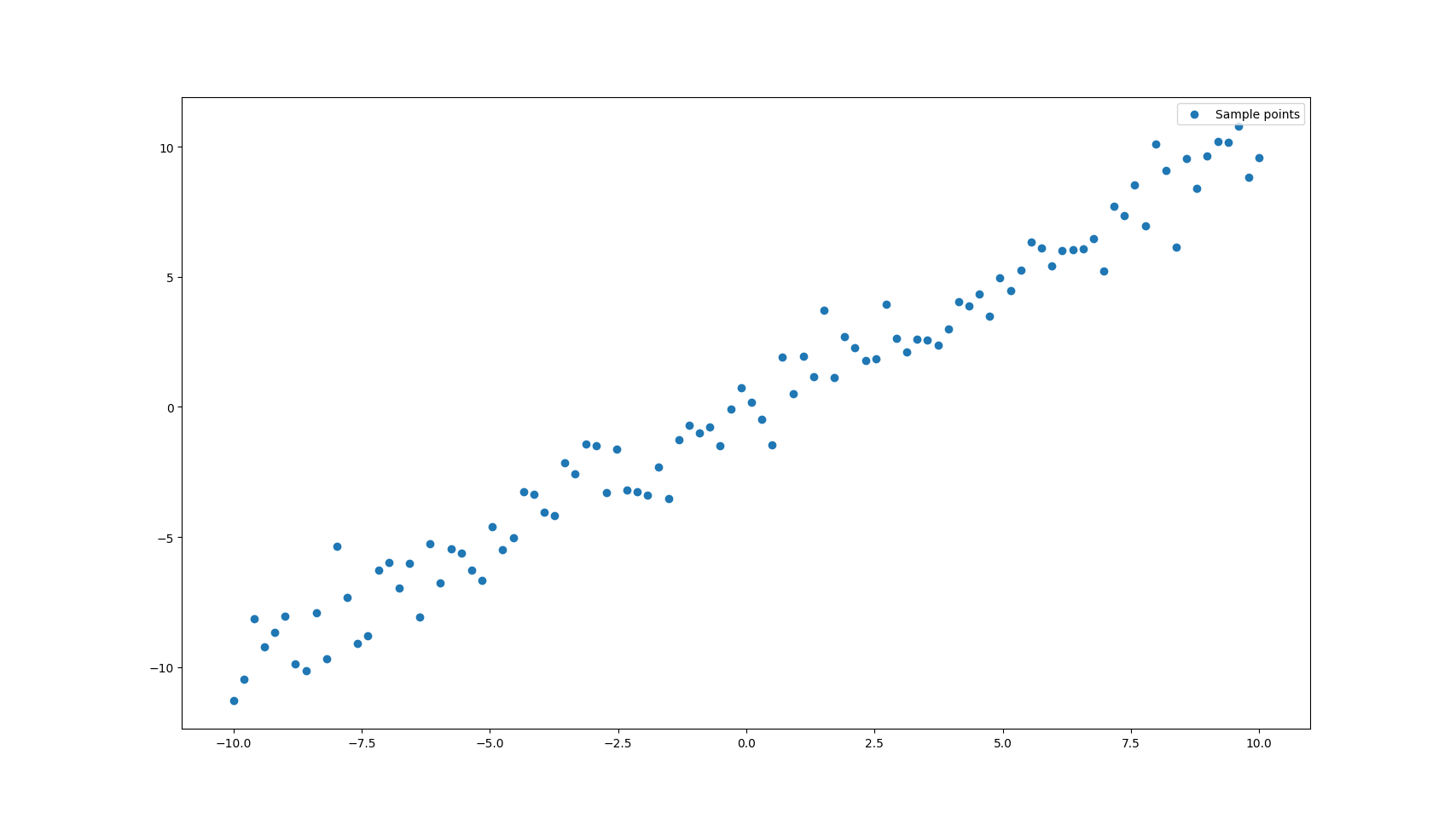

Looking at the plot, what we want to find is the general direction in which the points are spread. In other words, we want to capture the direction of maximum variance, which is exactly what SVD gives us. When we factorise $A = U \Sigma V^T$, if we take a column vector of V (called right singular vector) corresponding to the biggest singular value $\sigma_i \in \Sigma$, we get the direction of maximum variance.

Steps:

1. Center the points.
2. Compute SVD of $n$ points. i.e, for a $n$ point matrix $P \in \mathcal{R}^{n \times 3}$, we decompose into $P = U \Sigma V^T$ where $U \in \mathcal{R}^{n \times n}$, $\Sigma \in \mathcal{R}^{n \times 3}$ and $V^T \in \mathcal{R}^{3 \times 3}$.
3. We take the first row of $V^T$ (or first column of $V$), which corresponds to the biggest singular value in $\Sigma$ (in most of the libraries)

def fit_line(points):
    # Points: (n, 2)
    C = np.mean(points, axis=0)
    points_centered = points - C
    U, D, Vt = np.linalg.svd(points_centered)
    # The rows of Vt are the right singular vectors of 'points_centered'
    # First vector corresponds to the highest variance, thus gives the line.
    line = Vt[0]
    line = line / np.linalg.norm(line)

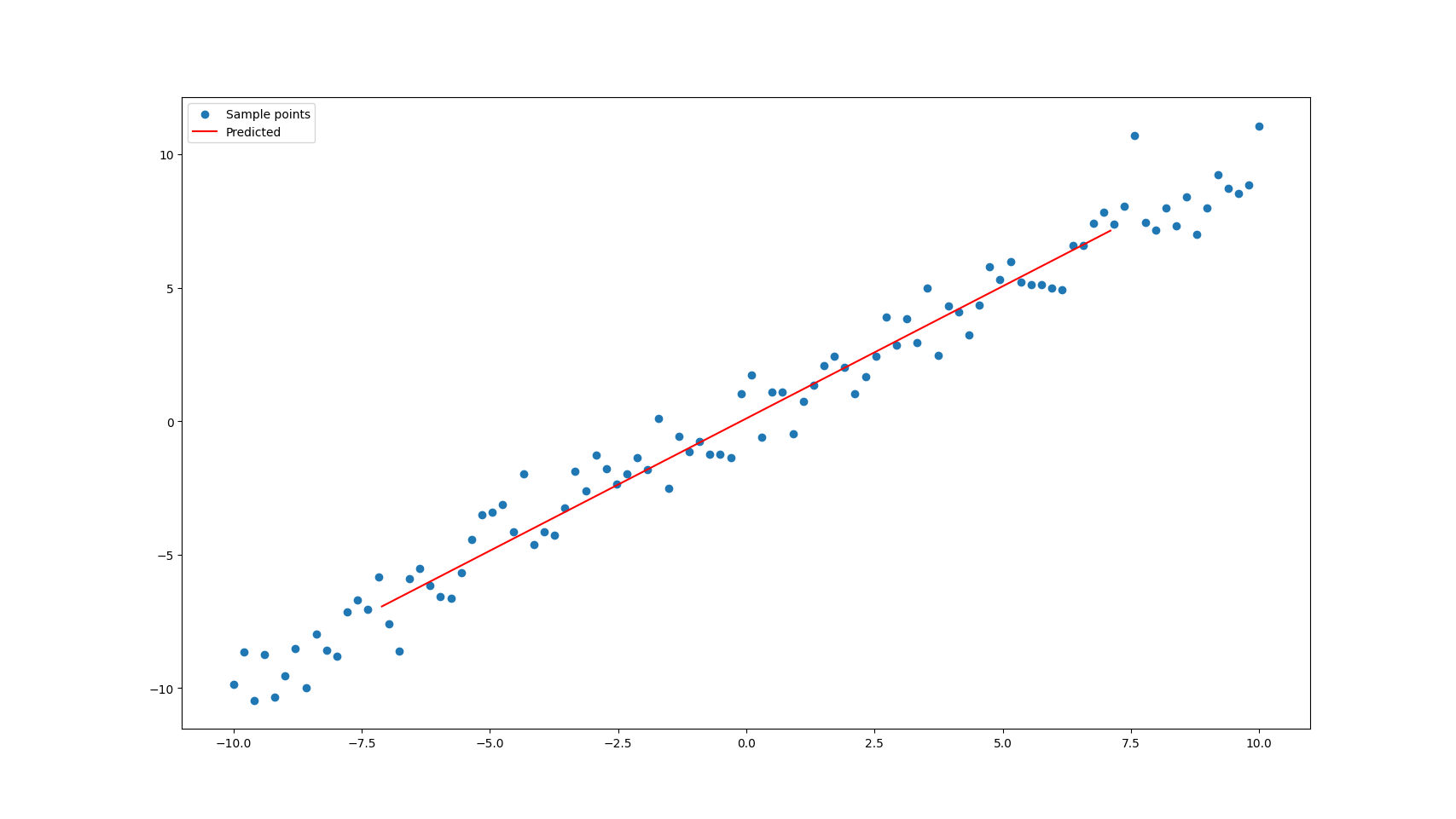
    return C, line

And if we plot the line we get,

Fitting a plane

The process of fitting a plane to 3D points is very similar to fitting a line. Instead of finding one direction of maximum variance, we’ll find two directions that define our plane.

Let’s first generate some sample 3D points that roughly lie on a plane:

def generate_plane_points(a, b, c, n_points, noise_std):
    xx, yy = np.meshgrid(np.linspace(-10, 10, n_points), np.linspace(-10, 10, n_points))
    zz = a * xx + b * yy + c
    noise = np.random.normal(0, noise_std, size=xx.shape)

    return xx, yy, zz, noise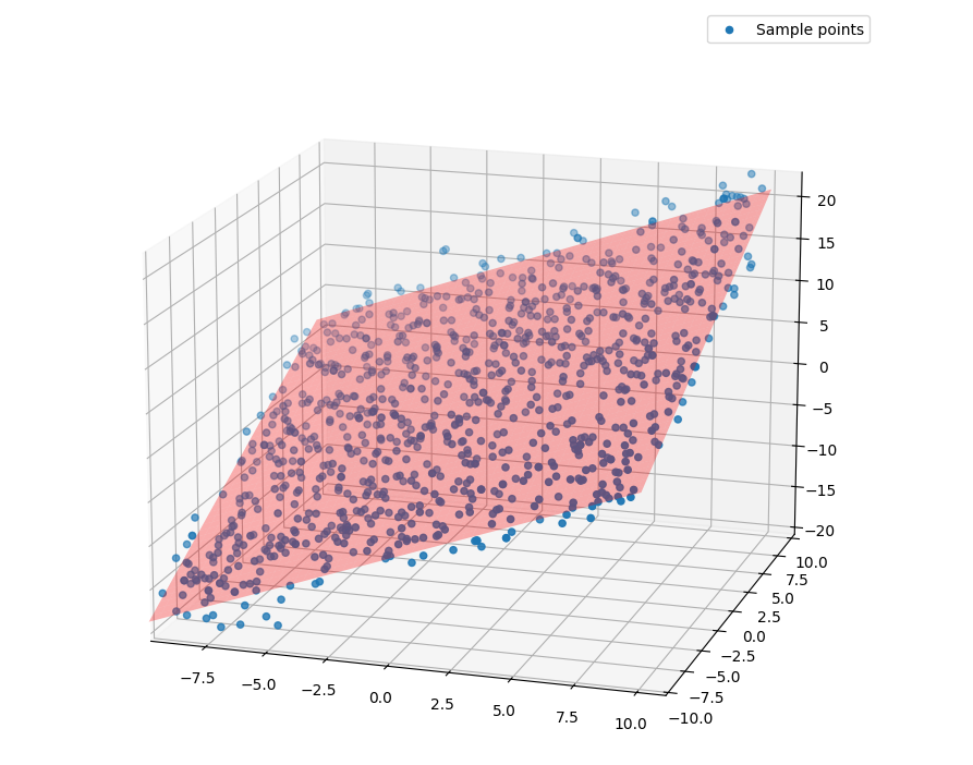

The steps to fit a plane are almost identical to fitting a line:

1. Center the points by subtracting their mean
2. Compute SVD of the centered points
3. The difference is that now we use the last right singular vector (corresponding to the smallest singular value), which gives us the normal vector to our plane. As we know the first 2 singular values correspond to higher variance, thus they should be the axes of the plane itself. Since a plane is normally defined by an origin and a normal, we can take the normal using the singular vector corresponding to smallest singular value.

Here’s the implementation:

def fit_plane(points):
    # Points: (n, 3)
    C = np.mean(points, axis=0)
    points_centered = points - C
    U, D, Vt = np.linalg.svd(points)
    # The rows of Vt are the eigen vectors of 'points_centered'
    # First two vectors with the highest variance, thus in plane.
    # Last vector will be the normal vector of the plane.
    normal = Vt[-1]
    normal = normal / np.linalg.norm(normal)

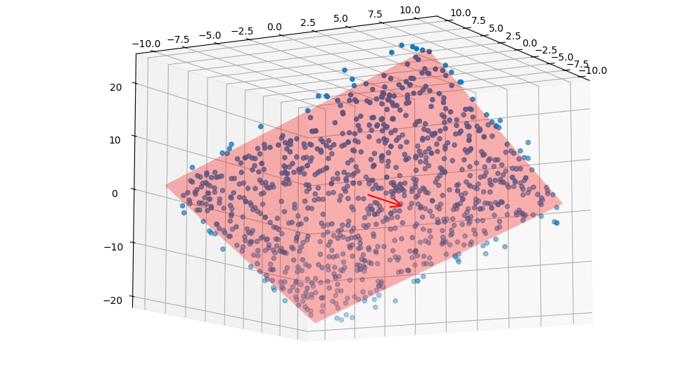
    return C, normal

When we visualize the result:

Why this works

In both cases (line and plane fitting), SVD helps us find the directions of maximum and minimum variance in our data:

• For line fitting, we use the direction of maximum variance (first singular vector)
• For plane fitting, we use the direction of minimum variance (last singular vector) as the plane normal

This approach is not only elegant but also robust to noise in the data. It minimizes the sum of squared perpendicular distances from the points to the fitted line or plane, which is exactly what we want in a “best fit” solution.

Interesting things to consider

1. Is this is the most efficient? We are doing SVD on $n \times 3$ matrix, just to get 3 components.
2. Why do we center points?