Matrix Calculus This post is a summary of The Matrix Calculus You Need For Deep Learning
Review: Scalar Calculus
Rule f ( x ) f(x) f ( x ) f ′ ( x ) f'(x) f ′ ( x ) Constant c c c 0 0 0 Multiplication by constant c x cx c x c c c Power rule x n x^n x n n x n − 1 nx^{n-1} n x n − 1 Sum rule f + g f + g f + g f ′ + g ′ f' + g' f ′ + g ′ Product rule f ⋅ g f \cdot g f ⋅ g f ⋅ g ′ + g ⋅ f ′ f\cdot g' + g\cdot f' f ⋅ g ′ + g ⋅ f ′ Quotient rule f g \frac{f}{g} g f f ′ ⋅ g − g ′ ⋅ f g 2 \frac{f'\cdot g - g'\cdot f}{g^2} g 2 f ′ ⋅ g − g ′ ⋅ f Chain rule f ( g ) f(g) f ( g ) f ′ ( g ) ⋅ g ′ f'(g) \cdot g' f ′ ( g ) ⋅ g ′
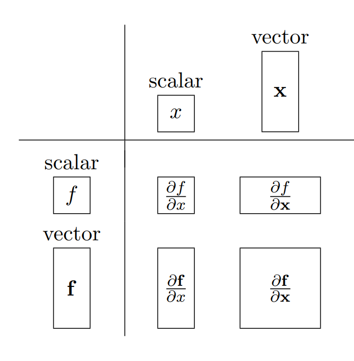
Introduction to Vector Calculus and Partial derivatives
Most “functions” in deep learning are influenced by multiple variables. And the way we describe the derivative / change of the function with respect to each variable is called the partial derivative . Consider the function f ( x , y ) f(x, y) f ( x , y ) ∂ f ( x , y ) ∂ x \frac{\partial f(x, y)}{\partial x} ∂ x ∂ f ( x , y ) ∂ f ( x , y ) ∂ y \frac{\partial f(x, y)}{\partial y} ∂ y ∂ f ( x , y )
For a single function, for eg. f ( x , y ) = 3 x 2 y f(x, y) = 3x^2y f ( x , y ) = 3 x 2 y
∂ f ( x , y ) ∂ x = 6 x y , ∂ f ( x , y ) ∂ y = 3 x 2 \frac{\partial f(x, y)}{\partial x} = 6xy ,\quad
\frac{\partial f(x, y)}{\partial y} = 3x^2 ∂ x ∂ f ( x , y ) = 6 x y , ∂ y ∂ f ( x , y ) = 3 x 2 and can arrange them in a vector form
∇ f = [ ∂ f ( x , y ) ∂ x ∂ f ( x , y ) ∂ y ] = [ 6 x y 3 x 2 ] \nabla f = \begin{bmatrix}
\frac{\partial f(x, y)}{\partial x} \\
\frac{\partial f(x, y)}{\partial y} \\
\end{bmatrix}
= \begin{bmatrix}
6xy \\
3x^2 \\
\end{bmatrix} ∇ f = [ ∂ x ∂ f ( x , y ) ∂ y ∂ f ( x , y ) ] = [ 6 x y 3 x 2 ] And when we want to find gradient for more than one function, say another function g ( x , y ) = 2 x + y 8 g(x, y) = 2x + y^8 g ( x , y ) = 2 x + y 8
∇ g = [ ∂ g ( x , y ) ∂ x ∂ g ( x , y ) ∂ y ] = [ 2 8 y 7 ] \nabla g = \begin{bmatrix}
\frac{\partial g(x, y)}{\partial x} \\
\frac{\partial g(x, y)}{\partial y} \\
\end{bmatrix}
= \begin{bmatrix}
2 \\
8y^7 \\
\end{bmatrix} ∇ g = [ ∂ x ∂ g ( x , y ) ∂ y ∂ g ( x , y ) ] = [ 2 8 y 7 ] And we can organize these two in a matrix form
J = [ ∇ f ( x , y ) ∇ g ( x , y ) ] = [ ∂ f ( x , y ) ∂ x ∂ f ( x , y ) ∂ y ∂ g ( x , y ) ∂ x ∂ g ( x , y ) ∂ y ] = [ 6 x y 3 x 2 2 8 y 7 ] J = \begin{bmatrix}
\nabla f(x, y) \\
\nabla g(x, y) \\
\end{bmatrix}
= \begin{bmatrix}
\frac {\partial f(x, y)}{\partial x} & \frac {\partial f(x, y)}{\partial y} \\
\frac {\partial g(x, y)}{\partial x} & \frac {\partial g(x, y)}{\partial y} \\
\end{bmatrix}
= \begin{bmatrix}
6xy & 3x^2 \\
2 & 8y^7 \\
\end{bmatrix} J = [ ∇ f ( x , y ) ∇ g ( x , y ) ] = [ ∂ x ∂ f ( x , y ) ∂ x ∂ g ( x , y ) ∂ y ∂ f ( x , y ) ∂ y ∂ g ( x , y ) ] = [ 6 x y 2 3 x 2 8 y 7 ] This is called Jacobian Matrix . This particular form is called Numerator layout , and its transpose is called Denominator layout . (Probably because the numerator of partial remains same in a row)
Generalisation of Jacobian Matrix
Instead of writing multiple variables, we can write them in a single vector. So, f ( x 1 , x 2 , x i . . . , x n ) = f ( x ) f(x_1, x_2, x_i ..., x_n) = f(\mathbf{x}) f ( x 1 , x 2 , x i ... , x n ) = f ( x ) f i f_i f i y i y_i y i f 1 , f 2 , . . . , f m f_1, f_2, ..., f_m f 1 , f 2 , ... , f m y \mathbf{y} y
y 1 = f 1 ( x ) y 2 = f 2 ( x ) ⋮ y m = f m ( x ) y_1 = f_1(\mathbf{x}) \\
y_2 = f_2(\mathbf{x}) \\
\vdots \\
y_m = f_m(\mathbf{x}) y 1 = f 1 ( x ) y 2 = f 2 ( x ) ⋮ y m = f m ( x ) And taking Jacobian,
J = ∂ y ∂ x = [ ∇ f 1 ( x ) ∇ f 2 ( x ) ⋮ ∇ f m ( x ) ] = [ ∂ f 1 ( x ) ∂ x 1 ∂ f 1 ( x ) ∂ x 2 ⋯ ∂ f 1 ( x ) ∂ x n ∂ f 2 ( x ) ∂ x 1 ∂ f 2 ( x ) ∂ x 2 ⋯ ∂ f 2 ( x ) ∂ x n ⋮ ⋮ ⋱ ⋮ ∂ f m ( x ) ∂ x 1 ∂ f m ( x ) ∂ x 2 ⋯ ∂ f m ( x ) ∂ x n ] J = \frac{\partial \mathbf{y}}{\partial \mathbf{x}}
= \begin{bmatrix}
\nabla f_1(\mathbf{x}) \\
\nabla f_2(\mathbf{x}) \\
\vdots \\
\nabla f_m(\mathbf{x}) \\
\end{bmatrix}
= \begin{bmatrix}
\frac{\partial f_1(\mathbf{x})}{\partial x_1} & \frac{\partial f_1(\mathbf{x})}{\partial x_2} & \cdots & \frac{\partial f_1(\mathbf{x})}{\partial x_n} \\
\frac{\partial f_2(\mathbf{x})}{\partial x_1} & \frac{\partial f_2(\mathbf{x})}{\partial x_2} & \cdots & \frac{\partial f_2(\mathbf{x})}{\partial x_n} \\
\vdots & \vdots & \ddots & \vdots \\
\frac{\partial f_m(\mathbf{x})}{\partial x_1} & \frac{\partial f_m(\mathbf{x})}{\partial x_2} & \cdots & \frac{\partial f_m(\mathbf{x})}{\partial x_n} \\
\end{bmatrix} J = ∂ x ∂ y = ∇ f 1 ( x ) ∇ f 2 ( x ) ⋮ ∇ f m ( x ) = ∂ x 1 ∂ f 1 ( x ) ∂ x 1 ∂ f 2 ( x ) ⋮ ∂ x 1 ∂ f m ( x ) ∂ x 2 ∂ f 1 ( x ) ∂ x 2 ∂ f 2 ( x ) ⋮ ∂ x 2 ∂ f m ( x ) ⋯ ⋯ ⋱ ⋯ ∂ x n ∂ f 1 ( x ) ∂ x n ∂ f 2 ( x ) ⋮ ∂ x n ∂ f m ( x )
Hessian Matrix
For a scalar function f ( x ) : R n → R f(\mathbf{x}): R^n \to R f ( x ) : R n → R
H = [ ∂ 2 f ( x ) ∂ x 1 2 ∂ 2 f ( x ) ∂ x 1 ∂ x 2 ⋯ ∂ 2 f ( x ) ∂ x 1 ∂ x n ∂ 2 f ( x ) ∂ x 2 ∂ x 1 ∂ 2 f ( x ) ∂ x 2 2 ⋯ ∂ 2 f ( x ) ∂ x 2 ∂ x n ⋮ ⋮ ⋱ ⋮ ∂ 2 f ( x ) ∂ x n ∂ x 1 ∂ 2 f ( x ) ∂ x n ∂ x 2 ⋯ ∂ 2 f ( x ) ∂ x n 2 ] H = \begin{bmatrix}
\frac{\partial^2 f(\mathbf{x})}{\partial x_1^2} & \frac{\partial^2 f(\mathbf{x})}{\partial x_1 \partial x_2} & \cdots & \frac{\partial^2 f(\mathbf{x})}{\partial x_1 \partial x_n} \\
\frac{\partial^2 f(\mathbf{x})}{\partial x_2 \partial x_1} & \frac{\partial^2 f(\mathbf{x})}{\partial x_2^2} & \cdots & \frac{\partial^2 f(\mathbf{x})}{\partial x_2 \partial x_n} \\
\vdots & \vdots & \ddots & \vdots \\
\frac{\partial^2 f(\mathbf{x})}{\partial x_n \partial x_1} & \frac{\partial^2 f(\mathbf{x})}{\partial x_n \partial x_2} & \cdots & \frac{\partial^2 f(\mathbf{x})}{\partial x_n^2} \\
\end{bmatrix} H = ∂ x 1 2 ∂ 2 f ( x ) ∂ x 2 ∂ x 1 ∂ 2 f ( x ) ⋮ ∂ x n ∂ x 1 ∂ 2 f ( x ) ∂ x 1 ∂ x 2 ∂ 2 f ( x ) ∂ x 2 2 ∂ 2 f ( x ) ⋮ ∂ x n ∂ x 2 ∂ 2 f ( x ) ⋯ ⋯ ⋱ ⋯ ∂ x 1 ∂ x n ∂ 2 f ( x ) ∂ x 2 ∂ x n ∂ 2 f ( x ) ⋮ ∂ x n 2 ∂ 2 f ( x ) ( H f ) i , j = ∂ 2 f ( x ) ∂ x i ∂ x j (H_f)_{i, j} = \frac{\partial^2 f(\mathbf{x})}{\partial x_i \partial x_j} ( H f ) i , j = ∂ x i ∂ x j ∂ 2 f ( x ) Important Matrix derivatives
Function Derivative ∇ x c \nabla_x c ∇ x c 0 ∇ x ( x + y ) \nabla_x (x + y) ∇ x ( x + y ) I I I ∇ y ( x − y ) \nabla_y (x - y) ∇ y ( x − y ) − I -I − I ∇ x ( f ( x ) T g ( x ) ) \nabla_x (f(x)^T g(x)) ∇ x ( f ( x ) T g ( x )) ( ∇ x f ( x ) ) g ( x ) + ( ∇ x g ( x ) ) f ( x ) (\nabla_x f(x)) g(x) + (\nabla_x g(x)) f(x) ( ∇ x f ( x )) g ( x ) + ( ∇ x g ( x )) f ( x ) ∇ x A x \nabla_x Ax ∇ x A x A T A^T A T ∇ x x T A x \nabla_x x^TAx ∇ x x T A x ( A T + A ) x (A^T + A)x ( A T + A ) x ∇ x g ( f ( x T ) ) \nabla_x g(f(x^T)) ∇ x g ( f ( x T )) ( ∇ x f T ) ∇ f g (\nabla_x f^T) \nabla_f g ( ∇ x f T ) ∇ f g
References
https://www.youtube.com/watch?v=ny-i8_9NtHA
https://ccrma.stanford.edu/~dattorro/matrixcalc.pdf